Whenever a scientist retires, resigns, is made redundant in their mid-50s, or leaves science for any reason there is a great deal of knowledge, know-how and wisdom lost.
I’m proposing an institute where these people are paid to come in a few days a month and thrash out their old theories for the benefit of younger scientists and engineers. There will be access to equipment, testing rigs and all sorts of analytical equipment, with free tea, coffee and biscuits. The full-time junior staff will be specially selected for their intelligence and patience.
One of my theories about innovation is that there are many half-notions in the world, but connecting your half to someone else’s half and making that bridge the gap between problem and solution can be a hit-and-miss affair. If you’ve ever heard something at random that sparks a memory and makes you go “Ah!” then you’ve bridged that gap.
Comedy writers are excellent at this, a joke is two ideas put together in an unexpected way.
The SIMOF solution is to have people who spent a lifetime bridging gaps create sparks in ways that nobody – least of all themselves – could anticipate.
It needs funding, and a site that has good access for public transport. Other than that, the idea’s good to go.
An experiment with bourbon may explain the high reputation of Japan’s whiskies
During my research for an earlier chemistry of whisky article, I came across an account of an experiment on how transporting barrels impacts the flavour of bourbon. Bourbon barrels are commonly used to age whisky not only in Scotland, but in England, Ireland, Japan and India.
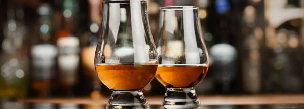
Whisky in Glencairn glasses. These glasses were developed in the early 2000s, inspired by the shape of the whisky blender’s glass.
I’d been looking at how the flavours of charred oak affect the character of bourbon. This article in Wine Enthusiast drew my interest. It described a fascinating experiment by Trey Zoeller, the founder of Jefferson’s bourbon distillery in Kentucky, USA. I originally put it in a footnote, but the whole thing became a bit extended and so I decided to convert it into an article.
Barrel aging bourbon
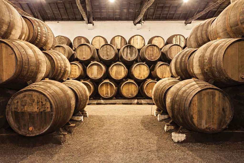
The usual practice when aging whisky/ whiskey1 is to have the barrels stacked in a warehouse holding maybe 60,000 barrels with 200 litres in each and let nature take its course.
Since 2012 Jefferson’s, based in Kentucky, has offered a limited ‘Ocean Cask’ expression. They send the barrels on six-month voyages at sea, where they are heated, chilled and shaken about before coming back to Kentucky to be bottled. Exact numbers of barrels aren’t available, but multiple shipping containers with 200 barrels each are now sent on these voyages. The 200-300 bottles that are filled from each barrel retail at $83 (about £60)2 for a 750 ml bottle, more than double their standard bourbon ($31).
Without good roads, the best option was for distillers to send barrels down the Mississippi with the spring flood, then by ship from New Orleans to New York for bottling. In 2022, Jefferson’s sent two barrels of bourbon on a replica journey down the Mississippi and then to New York to see if this process was the source of Kentucky bourbon’s high reputation.
A barge on the Mississippi.
The agitation of the spirit in the barrel during transit did change the flavour, both chemical analysis and blind tasting showed a distinct variation. This could explain the good reputation that Kentucky bourbon enjoyed in New York.
Relevance to whisky
Bourbon is similar to whisky, in that you take a grain-derived spirit and age it in wooden barrels until it has absorbed flavours from the barrels and the environment. The difference is the type of grain you use. Malt whisky is made using barley. By law, bourbon must contain over 51% corn grain spirit. Anything else is grain whisky3.
As my previous blog discussed, a lot of whisky is aged in used bourbon barrels. The environment in which the whisky aging takes place influences the flavours extracted from the wood. Bourbon is produced in the generally temperate continental climate of Kentucky, so the mix of grains (the ‘mash bill’), the type of still used and the cut of the spirit are more important in determining the particular flavour4 of the bourbon.
The flavours extracted from used bourbon barrels by the maturing whisky will be representative of the original spirit. The mix of flavour molecules extracted will also vary depending on several factors including the ethanol content of the whisky, temperature, humidity, and time.
Scotland is a cool, damp country and produces characteristic whisky. By law whisky must be aged for at least three years to be sold as Scottish whisky. Age adds to the flavour, smoothness and cost of a whisky. The oldest whisky I’ve ever has is a 20 year old Highland Park – a slightly peaty but incredibly smooth drink that cost about £25 for a double5.
Japan and the getting back to the point
All this is fine, but what does the Jefferson bourbon experiment have to do with whisky? After all, shipping or moving thousands of heavy barrels isn’t a commercially viable option unless you’re going to add a premium to an already expensive product.
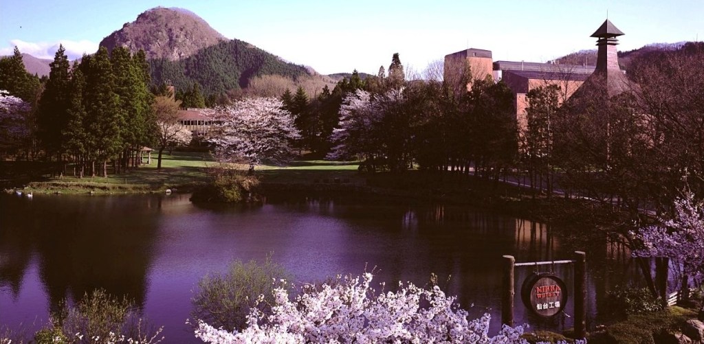
Japan has a well-established whisky manufacturing culture, with the first whisky distillery – Suntory – opening near Kyoto in 1923. Following a disagreement between the founders, a second distillery, Nikka, was opened near Sapporo on the north island of Hokkaido. This site was chosen because the climate was more like Scotland than the sub-tropical Kyoto.
The Nikka distillery near Sapporo. A new place I want to visit, it looks lovely.
Japan’s whisky industry was established after thoroughly researching the Scottish methods and equipment, even buying old stills from distilleries and, in places, a climate that mimics that of Scottish. From those beginning decades ago, Japanese distilleries have developed the craft to produce a distinct drink that has its own place in the world of whisky.
What is perhaps unique in Japan is that is a whisky-producing country that also sits on a tectonically active region, at the junction of at least three active geological faults. Low intensity tremors are frequent throughout the islands with major quakes occurring annually.
So, while shipping thousands of barrels by sea to enhance the extraction of flavours isn’t economically feasible, it could be that the character of Japanese whisky is changed through frequent shaking by earthquakes. It could be that, in their quest to create a Scottish whisky with a Japanese feel, the geology of their country has gifted the Japanese whisky industry an added influence that the distillers of other countries will find it difficult to emulate.
Traditionally, whisky is from Scotland, whiskey isn’t. Though some Japanese distilleries use ‘whisky’. ↩︎
I had to enter an address in the USA to get this price. I picked 1060 West Addison St, Chicago. ↩︎
Quinoa can be used to make whisky, even though it’s not technically a grain. ↩︎
Saturn’s sixth-largest moon may have the right conditions for life. But how to prove if there is life on Encaladus?
Background – Cassini-Huygens mission
The Cassini-Huygens mission was launched in 1997 with the mission objective to explore the saturnian system. It would take seven years to reach Saturn, and it would collect images, chemical analyses and magnetic field readings as it passed through the inner solar system, the asteroid belt and past Jupiter.
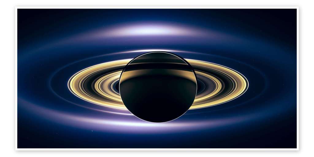
Image of Saturn eclipsing Cassini.
This would be the first mission to orbit Saturn and would carry the Huygens lander, which landed on Saturn’s largest moon, Titan. Among the instruments on the Cassini probe there was a mass spectrometer, the Cosmic Dust Analyzer1, which was designed to collect and characterise cosmic dust.
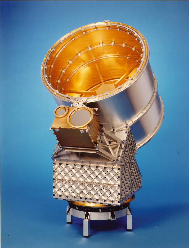
The Cosmic Dust Analyzer (CDA) that was mounted on the Cassini probe. The opening is about 40 cm, the hexagon in the middle is the multiplier, which sits above the ionisation grid. The detectors are at the bottom of the cylinder, hidden from view. The unit is mounted on a turntable which allowed it to collect dust from a wider angle than if it had been stationary.
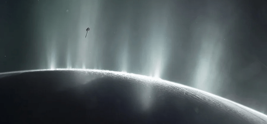
Among the many amazing discoveries on the mission was the observation of gas plumes – cryovolcanoes – erupting from the southern polar region of Enceladus, the sixth-largest of Saturn’s 274 moons2 .
Further observation and analysis of the plumes showed that they were mostly water and these ice crystals also constituted much of Saturn’s E-ring, the fifth ring to be discovered, whose existence was not confirmed until 1980.
Astronomers reached this conclusion from the chemical analysis provided by the CDA in the early part of the mission. Collecting dust from the E-ring and from around Enceladus, it was seen that the chemical make-up of the ice crystals in the ring and in the plumes matched. However, looking again at the chemicals trapped inside it was concluded that the water coming out of Enceladus was salty and contained not only silicates, but ammonia and organic chemicals of varying complexity.
A recent publication in Nature Astronomy3 has summarised the analysis of data collected by the Cosmic Dust Analyzer (CDA) during the last part of the probe’s orbit of Saturn from 2004 to 2017. The organic chemistry observed in these analyses shed light on the make-up of the oceans of Enceladus and raised the possibility that the moon is capable of supporting life.
The first question that needs to be asked in the search for extra-terrestrial life is whether the conditions are suitable for life to exist. Liquid water at a reasonable temperature and pH is one such condition4. Also, six elements – carbon, hydrogen, oxygen, nitrogen, phosphorus and sulphur – are regarded as necessary for biological systems to survive.
Enceladus
Enceladus was discovered by William Herschel in 1789. Not much was known about it before the Cassini mission. It was known that it was 500 km in diameter – one seventh the size of our moon – and was associated with Saturn’s E-ring, though how the two interacted was not known.
Enceladus, photographed by Cassini. The fissures cover most of the moon’s surface, except in the southern region. A small proportion of the ice from the plumes falls back to the moon and covers this region in smooth snow.
Analysis of the magnetic data that Cassini collected provided astronomers with a update on the structure of the moon. There is a rocky core and an icy upper crust – this much was known. But data strongly suggested that there is a liquid ocean between the rock and the ice. This is a salty, high pH (11 to 12) environment but crucially there is liquid water.
The article by Khawaja et al provides an analysis of some of the data the CDA collected in the last months of the mission. It has taken years to refine the data to the point where statistically significant conclusions can be drawn. A lot of the information from the Cassini fly-past was collected at relatively slow speeds. And ‘relatively’ means less than 12 km/s. Data from higher speed fly-bys at up to 18 km/s were also collected and form the basis of the new analysis.
The speed at which the crystals were collected matters. The way the CDA works is that the crystals would hit a screen at the front of the CDA. The crystals are tiny – at most 1 nanometre (one millionth of a micrometre) and some ten orders of magnitude smaller (10-19 m)5. In the time it takes the ionised particles to reach the detector (about 20 microseconds at lower speeds) the water will freeze and this can shield many of the analytes from the instrument. At higher impact speeds the ice did not have time to reform and so more of the trapped chemicals were visible to the detector.
With faster incoming particles, the detector had to work faster to be able to distinguish between each particle. Higher speed detection required the analyser to work at its maximum rate and in a mode for which it was not really designed. The data were noisy and in the years since a great deal of effort has been spent finding enough useful data to be able to make conclusions.
What was found was some volatile organics such as methane and ethane, plus a mix of volatile low-mass nitrogen and oxygen bearing organics, single-ring aromatics and some complex macromolecular species, up to the limit of detection of the CDA (about 200 Da).
This complex mix of chemicals can be seen as the building blocks for life and raises the question of what the source of these chemicals could be.
In all this, you have to bear in mind that the CDA was designed and built nearly 30 years ago. Computer speeds have increased massively since the mid 90s and a CDA designed now would be smaller and more efficient than the one on Cassini. But also a CDA built in 2055 would be more advanced again.
James Webb
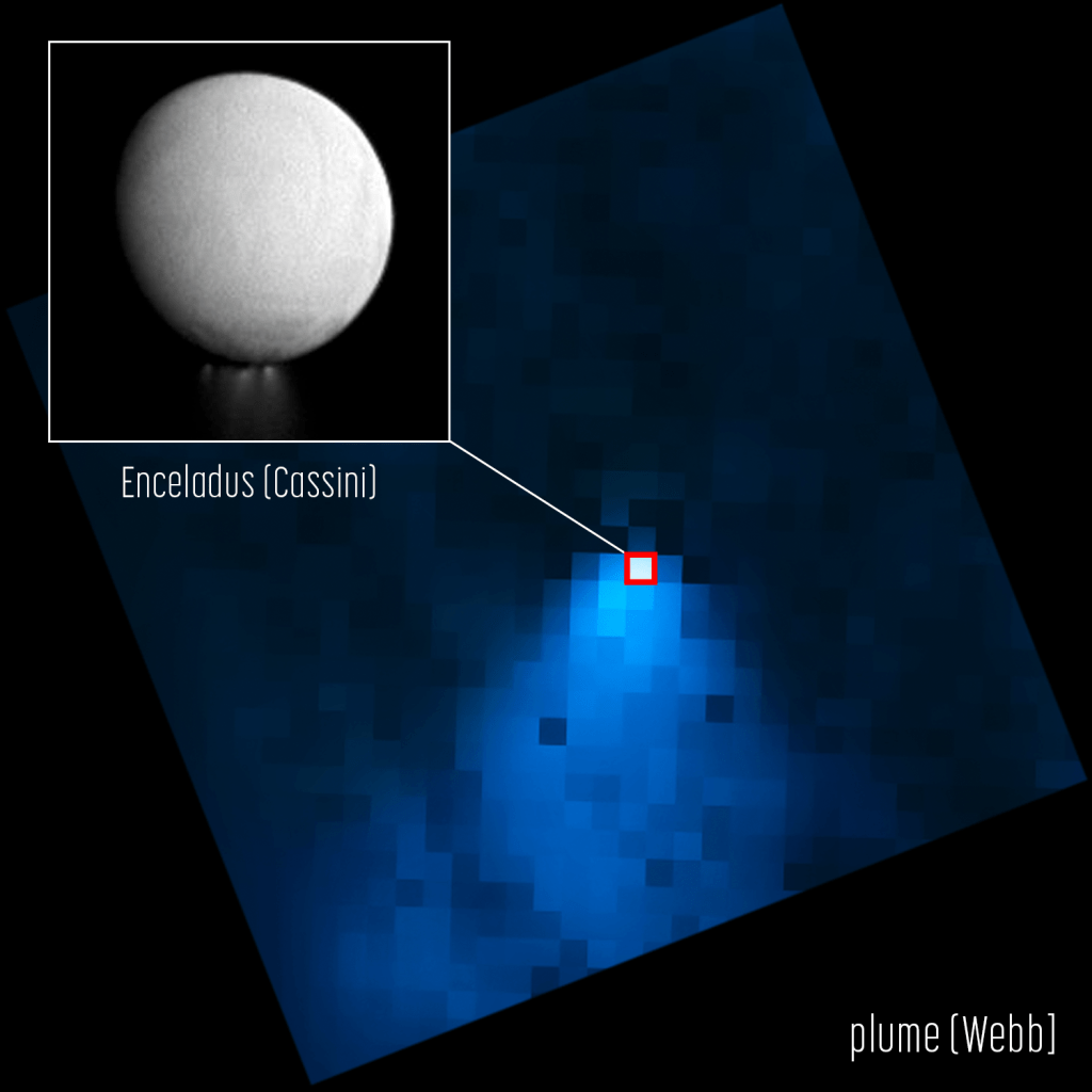
The James Webb telescope, launched in 2021, has investigated Enceladus. Using near infrared – more sensitive to water than the instruments on Cassini – it detected water plumes extending 10 000 km from the moon. Enceladus itself is only 500 km in diameter.
Near-infra red image from the James Webb telescope. The blue colour is water, almost all of which originates from Enceladus. The plume extends up to 10 000 km from the moon.
New missions to Enceladus have been proposed, but are not likely to take place any time in the next ten years. The tantalising possibility that there is life on another body of the solar system has taken a step closer with these data.
The mix of chemicals determined to be in the plumes, and therefore in the oceans of Enceladus, are known to be those that support life. Until or unless we get a sample of an enceladan microbe under a microscope there won’t be proof of life there. The data reported by Khawaja doesn’t mean that there is definitely life on Enceladus. It does mean that it’s possible.
Full description in Srama et al (2004) Space Science Reviews 114: 465-518 ↩︎
At the time of writing, there were 274 named moons. More may well be found in the coming years. ↩︎
The limits of ‘reasonable’ has changed over the last few decades. Extremophile microbes capable of surviving and thriving at temperatures of 120 °C and pH up to 11 have been found. ↩︎
This is a huge dynamic range for the detector to be able to analyse. It’s like being able to analyse a grain of sand and something the size of the Earth’s orbit in the same instrument. ↩︎
A slight departure, this time I’ve designed a mug. I was thinking about what molecules would look good on a coffee mug and the obvious answer was ‘caffeine’.
One of the things I had planned to use Blender for was to make scientific models and diagrams as well as protein and molecular models. How to do these things was another matter and how to make anything of them when the market for scientific diagrams is (a) small and (b) a closed shop were further matters.
Having had the idea of caffeine-on-a-mug1 I hit the University of YouTube and found out how to get from a molecule to a 3D design, and then from a 3D design to a cartoonised version. This latter was a design choice – I thought it would look bold and also it would be a way of cutting down on the number of colours required for the design.
I found a good tutorial by CG Figures who went through the two-step process to get from molecule name to a file that can be read by Blender.
I was already familiar with one of the websites that was recommended – molview.org – and the software to convert the SMILES file into a protein database (.pdb) file was easy enough to use. The SMILES format is a standardised way of representing organic molecules and it was the format I used to input molecules of interest into a molecular modelling tool to predict the pharmacokinetics of drugs – SwissADME is the website, if you’re interested.
Once I’d got the molecule model into Blender, there were a bunch of further steps to clean up the file into something that didn’t take up too much filespace and have extraneous faces that could give odd results when the image is finally rendered.
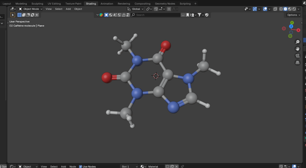
The caffeine molecule after some tweaking of the initial file. The software adds colours by default, in this case grey is carbon, blue is nitrogen, red is oxygen and white is hydrogen.
It didn’t take long to get to the point where I had a model that I could use as a basis for a design. Next, I wanted to turn it into a cartoon version. This means that the light and shade are demarcated by sharp lines with no fading.
In Blender there is a function called a “color ramp” which takes a colour or a shade and changes it. Using this I could control which parts of the atoms were darker and which had highlights. By moving the light around I could change where the light spots landed and also change the size of the highlights. And because the software sees the molecular model as a three dimensional object, the highlights vary around the model, making the model look more three dimensional, even though the idea is to create a two dimensional image.
Three cartoon monkey heads. Turning the head changes the cartoon lighting and adding grease pencil adds definition to the image.
In order to add a more cartoony look, a function called grease pencil can be used to add black lines to the scene. There are two ways to do this. Blender can add grease pencil automatically, which is what I’ve done here. You can also add it manually so that you can put details on the image.
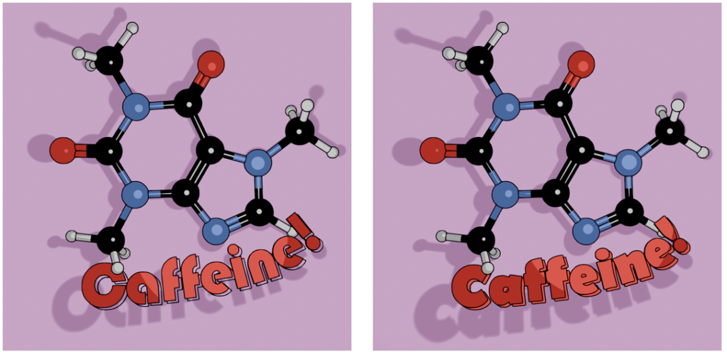
Anyway, back to the caffeine image. Not only did I add the cartoon effect and grease pencil, but the molecule needed a caption so we know what it is.
Alternative fonts for the caption. I like the Bauhaus font (left) as a design choice, but the capital C is a bit too closed to read easily. Berlin font (right) has a similar vibe and a more open C.
Looking through font choices I tried Bauhaus – it’s bold and has a historic feel to it. After showing this to Mrs S, I changed to Berlin. She pointed out that the C in the Bauhaus font is a bit too closed, and the Berlin version looks better in this application.
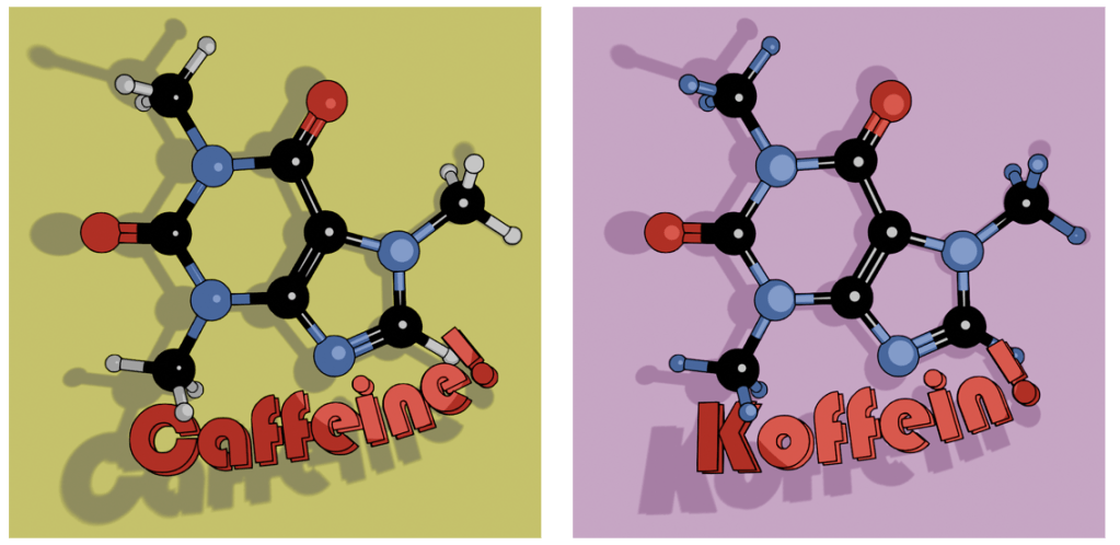
As an alternative, there’s also the molecule on a mustard-coloured background and in German. I’ve yet to offer these alternatives in the shop, I don’t know how big the German market for nerdy science mugs is2. I will likely keep the Bauhaus font for this, since the K looks echt cool, oder? I’ll need to use either Berlin or another font for the French (caféine), Spanish and Portuguese (cafeína) and Italian (caffeina) versions.
Two view of caffeine (Bauhaus font) and Koffein. Mustard yellow background or pinky purple? Which is better?
I can try other background colours, but I’m not sure what works best. Any suggestions are welcome.
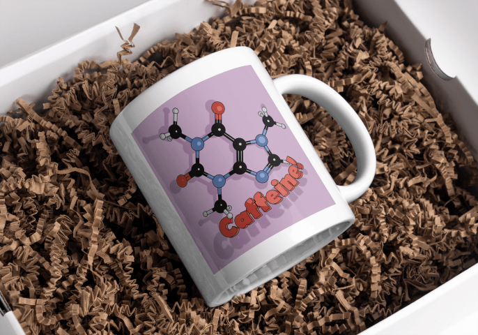
The finished design could then be uploaded to Gelato so I could put that onto a mug and then get it published on Etsy.
Mock-up of the finished mug nestled in a bed of curly brown stuff.
“We are about to jump into hyperspace for the journey to Barnard’s Star. On arrival we will stay in dock for a seventy-two-hour refit, and no one’s to leave the ship during that time. I repeat, all planet leave is cancelled. I’ve just had an unhappy love affair, so I don’t see why anybody else should have a good time.”
Cpt Prostetnic Vogon Jeltz, Hitchhiker’s Guide to the Galaxy
Over the last 20 years, thousands of exoplanets have been discovered (5867 in 4377 systems according to Wikipedia). The first confirmed exoplanet was announced in 1992, when planets were detected around a pulsar.
Pulsars are rotating neutron stars that emit a highly regular beam of electromagnetic radiation1. The pulses emitted by a pulsar with a planet are slightly altered by the presence of a gravitational field, such as that caused by the presence of a planet. It was anomalies in the pulse period of a pulsar in the constellation Virgo that led to the discovery of the first exoplanet. Or rather exoplanets, because this pulsar has three, including one that is half the mass of the Moon.
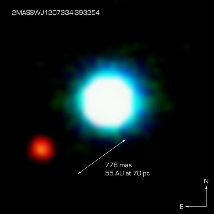
Direct imaging wasn’t really an option until much later. The first exoplanet to be directly imaged wasn’t announced until 2004, when 2M1207b was observed orbiting its parent star the brown dwarf 2M1207 (in the constellation Centaurus), 170 light years away by the Very Large Telescope in Chile.
First confirmed direct image of an exoplanet from the VLT in Chile. This is an infrared image of the brown dwarf and its planet.
To date (4th April 2025), 128 stars have had planets directly observed around them, (including one with four planets). Our closest star, Proxima Centauri, was shown to have a planetary system in 2016; a third planet was announced in 2022.
The Hubble telescope and, more recently, James Webb telescope have provided direct images of many more exoplanets. Spectroscopic analyses have given us insight into the atmospheres of some of the planets.
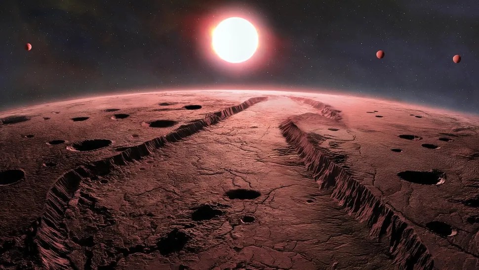
Barnard’s Star
Anyway, back to Barnard’s Star. This is one of the closest stars to Earth, though it is so faint that it wasn’t discovered until 1916, by Edward Barnard. He announced the discovery of a star with a large proper motion (how far it appears to travel) after observations 14 days apart. He followed this up with reference to observations made in 1894 (Lick Observatory in California) and 1904 (Bruce Observatory, Whitby), where the star showed up on earlier photographic plates. From this, he calculated a proper motion of 10.3″ a year, or one degree every 6 years.
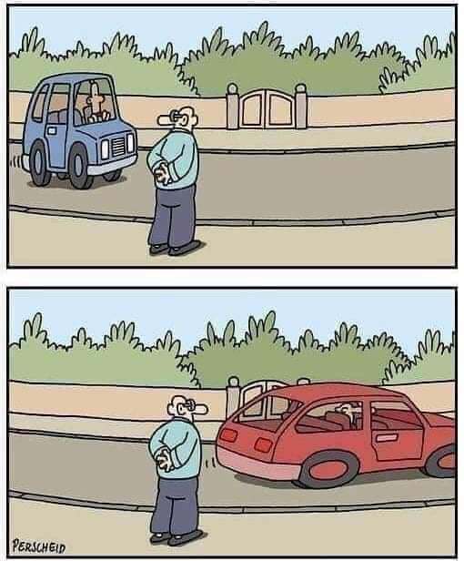
So it’s moving fast. And it’s getting closer. It’s one of the few objects in the sky with a blue shift — the most important other one is the Andromeda Galaxy, which is approaching the Milky Way at about 110 km/s; they are expected to collide in 4 to 5 billion years. Get your crash helmets ready.
Blue shift is the opposite of red shift. Light is ‘shifted’ when the expected spectrum of light from the star is different to what is expected from the known emission spectrum of the elements in the star. It’s also known as the Doppler Effect and is the basis of this cartoon by the German cartoonist Martin Perscheid.
Trust me, it’s funny.
So we have a star that’s approaching and it has at least four planets. Why the fuss? Well, there have been plans to visit either Barnard’s star or the Alpha Centauri system. Back in the late 1970s the idea was mooted to build a probe capable of travelling one-tenth the speed of light. The probe would take forty years to get there, and another four years before any signals from the probe arrived at Earth.
So we could now be getting images of planets from a probe that was launched before we even knew that these planets existed.
There’s some physics behind this that I don’t fully understand. ↩︎